RcTorch Tutorial: Forced Pendulum Example
Installation
Using pip
Like most standard libraries, RcTorch is hosted on [PyPI](https://pypi.org/project/RcTorch/). To install the latest stable release use pip:
pip install -U rctorch # '-U' means update to latest version
Imports
To import the RcTorch classes and functions use the following:
from rctorch import *
import torch
Load data
RcTorch has several built in datasets. Among these is the forced pendulum dataset. Here we demonstrate how the “forced pendulum” data can be loaded
fp_data = rctorch.data.load("forced_pendulum",
                             train_proportion = 0.2)

force_train, force_test = fp_data["force"]
target_train, input_test = fp_data["target"]

#Alternatively you can use sklearn's train_test_split.
Set up Hyper-parameters
Hyper-parameters, whether they are entered manually by the RcTorch software user or optimized by the RcBayes class (see the Bayesian Optimization section to see how to automatically tune hyper-parameters), are generally given to the network as a dictionary.
#declare the hyper-parameters
>>> hps = {'connectivity': 0.4,
           'spectral_radius': 1.13,
           'n_nodes': 202,
           'regularization': 1.69,
           'leaking_rate': 0.0098085,
           'bias': 0.49}
Setting up your very own RcNetwork
RcTorch has two principal python classes. The first is the RcNetwork class, which stands for “Reservoir Computer Network”, the long name being reservoir computer neural network.
An echostate network is the same thing as an RC network because another name for “Reservoir Computer” is “EchoState Network”
In order to use the fit :method: and the test :method:, we must first declare the RcNetwork object
my_rc = RcNetwork(**hps, random_state = 210, feedback = True)

#fitting the data:
my_rc.fit(y = target_train)

#making our prediction
score, prediction = my_rc.test(y = target_test)
my_rc.combined_plot()
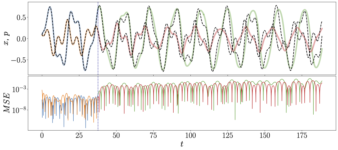
Feedback allows the network to feed in the prediction at the previous timestep as an input. This helps the RC to make longer and more stable predictions in many situations.
Setting up your very own Parameter Aware RcNetwork
Note
In Robotics and Control theory, an observer is a parameter which the user knows, even for future values. For example, we might know, or be able to control, how much a robot pushes on a pendulum. The time-series we know are called \(\text{observers}\), and all inputs (\(\texttt{X}\)) to RcTorch are treated as such.
Giving RcTorch inputs is easy! just supply an argument to \(\texttt{X}\).
my_rc = RcNetwork(**hps, random_state = 210, feedback = True)

#fitting the data:
my_rc.fit(X = force_train, y = target_train)

#making our prediction
score, prediction = my_rc.test(X = force_test, y = target_test)
my_rc.combined_plot()

Bayesian Optimization
Unlike most other reservoir neural network packages ours offers the automatically tune hyper-parameters.
In order to tune the hyper-parameters the user can use our RcBayesOpt class. The key argument to this class’s __init__() method is the bounds_dict argument. The keys of this bounds dict should be the key hyper-parameters of the model.
In particular, an overview of the main HPs used in this study is given by the Key Hyper-parameters used in RcTorch table below. Here \(N\) represents the total number of nodes in the reservoir. The spectral radius \(\rho\) is the maximum eigenvalue of the adjacency matrix, (the adjacency matrix determines the structure of the reservoir). The hyper-parameter \(\zeta\) is the connectivity of the adjacency matrix. The bias \(b_0\) used in the calculation of the hidden states and the leakage rate \(\alpha\) controls the memory of the network, i.e. how much the hidden state \(h_k\) depends on the hidden state \(h_{k-1}\). The ridge regression coefficient \(\beta\) determines the strength of regularization at inference (when solving, in one shot, for \(\bf{W}_{out}\) ).
\(\bf{\text{HP}}\) |
\(\bf{\texttt{RcTorch Variable name}}\) |
\(\bf{\text{Description}}\) |
\(\bf{\text{Search Space}}\) |
|---|---|---|---|
\(N\) |
\(\texttt{n_nodes}\) |
number of reservoir neurons |
typically 100 to 500 |
\(\rho\) |
\(\texttt{spectral_radius}\) |
Spectral radius max eigenvalue of \(\bf{W}_text{res}\) |
[0,1] |
\(\zeta\) |
\(\texttt{connectivity}\) |
connectivity of the reservoir (1 - sparsity) |
logarithmic |
\(\mathbf{b_0}\) |
\(\texttt{bias}\) |
bias used in the calculation of \(\mathbf{h_k}\) |
[-1,1] |
\(\alpha\) |
\(\texttt{leaking_rate}\) |
leakage rate |
[0,1] |
\(\beta\) |
\(\texttt{regularization}\) |
ridge regression coefficient |
logarithmic |
Setting up the RcBayesOpt object
#any hyper parameter can have 'log_' in front of it's name.
#RcTorch will interpret this properly.
bounds_dict = {"log_connectivity" : (-2.5, -0.1),
               "spectral_radius" : (0.1, 3),
               "n_nodes" : (300,302),
               "log_regularization" : (-3, 1),
               "leaking_rate" : (0, 0.2),
               "bias": (-1,1),
               }
rc_specs = {"feedback" : True,
             "reservoir_weight_dist" : "uniform",
             "output_activation" : "tanh",
             "random_seed" : 209}

rc_bo = RcBayesOpt(bounds = bounds_dict,
                    scoring_method = "nmse",
                    n_jobs = 1,
                    cv_samples = 3,
                    initial_samples= 25,
                    **rc_specs
                    )
Running the BO optimization
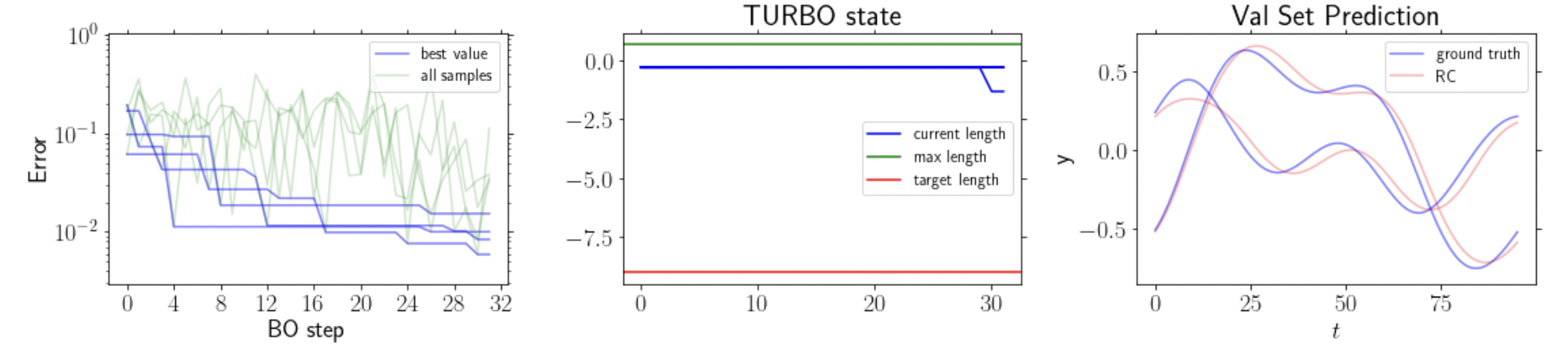
RcTorch uses a a special version of Bayesian Optimization known as TuRBO which can train many RCs at once. TuRBO runs multiple BO “arms” at once, essentially running local BO runs in parallel. RcTorch shows three panels to represent TuRBO training. The first panel shows the BO history, with all the BO scores in green and the minimum value in blue. The second panel shows the TuRBO convergence. The third panel shows the best BO prediction in the most recent round.
Running Bayesian Optimization (BO) with RcTorch is easy. We just need to run the optimize() method. The key arguments include n_trust_regions which determines the number of trust regions (parallel BO runs), the
max_evals argument which determines the maximum number of RCs to train, and the scoring_method which determines the RC loss function.
opt_hps = rc_bo.optimize( n_trust_regions = 4,
                                  max_evals = 500,
                                  x = force_train,
                                  scoring_method = "nmse",
                                  y = target_train)
The BO run returns a new set of HPs which we can use with a new RcNetwork.
#new_hps
>>> opt_hps = {'connectivity': 0.4,
           'spectral_radius': 1.13,
           'n_nodes': 202,
           'regularization': 1.69,
           'leaking_rate': 0.0098085,
           'bias': 0.49}